
|
What's Happened to Homeownership? In 1991, 64.1 percent of all American households owned their homes. This percentage remained virtually unchanged through 1994, when the homeownership rate was 64.0 percent. Since 1994, the homeownership rate has risen continuously and substantially so that, in 1999, 66.8 percent of all American households owned their homes. Using data from the American Housing Survey (AHS), this article examines how changes in homeownership rates for different groups led to the large increase in the national homeownership rate. There are two worthwhile reasons for looking at changes in homeownership rates for subgroups within the population. First, the subgroup experience can explain changes in the national rate. For example, because older households typically have higher homeownership rates, the aging of the population could produce an increase in the national homeownership rate without the homeownership rate of any age group increasing. Second, the suitability of any national homeownership rate depends in large part on how the national experience is shared by subgroups. The American dream of homeownership applies to the entire population, not just the average household. The Whole Is Equal to the Sum of Its Parts In comparing homeownership rates in different years, one can separate the influences of changing population characteristics and changing homeownership trends within the population by posing two questions:
In calculating homeownership rates to two decimal places, the AHS shows that the national homeownership rate increased by 1.62 percentage points between 1991 and 1997. The rate effect accounted for 1.37 percentage points or 85 percent of the increase. The composition effect accounted for 0.26 percentage point or 16 percent of the increase. Although the population changed in ways that enhanced homeownership during the 1990s, this effect was minor compared with the general improvement in rates for all groups. The AHS also shows that homeownership rates for minorities increased by 2.25 percentage points between 1991 and 1997.3 This increase was higher than the overall change. The rate effect for minorities was 1.52 percentage points or 68 percent of the increase. The composition effect was 0.73 percentage point or 32 percent of the increase. For whites, the homeownership rate increased by 2.60 percentage points between 1991 and 1997. The rate effect was 1.32 percentage points or 51 percent of the increase, and the composition effect was 1.28 percentage points or 49 percent of the increase. Between 1991 and 1997, the homeownership rate in central cities increased by 0.34 percentage point according to the AHS. However, the composition effect was negative, because population shifts alone should have reduced the central city homeownership rate by 1.43 percentage points. Instead, a 1.78- percentage-point rate effect offset the demographic trends and produced an increase in homeownership rates in central cities. There appears to have been a strong upward shift in homeownership rates throughout the population between 1991 and 1997. In most cases, this upward shift in rates added to favorable demographic trends; in other cases, it was strong enough to offset negative demographic trends. The rate effect was more important than the composition effect for minorities, whereas the two effects were approximately equal for whites.4 Have Gaps Narrowed? In the August 1994 issue of U.S. Housing Market Conditions, HUD showed that, within the structure of subgroup homeownership rates, there were substantial gaps between minorities and whites and among different income classes. Even controlling for age, income, and household type, minority homeownership rates were consistently lower than white homeownership rates. Similarly, after controlling for age, race, and household type, lower income households had lower homeownership rates than higher income households. The AHS can be used to show whether these gaps have been reduced and, if so, the extent to which a reduction comes from higher subgroup rates or simply demographic trends.
Table 1. Gaps in Homeownerships Rates by Income, 1991 an 1997 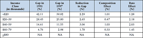 Table 1 shows this income gap as the difference in homeownership rate between each income class (measured in 1991 dollars) and the highest income group. For example, the homeownership rate in 1997 for households with incomes below $20,000 was 49.77 percent, and the rate for households earning $80,000 or more was 89.59 percent. This results in a gap of 39.82 percentage points. Table 2 shows that the gap for each income class declined between 1991 and 1997. In each case, the demographic trends contributed to the decline in the gap, but improvements in the underlying rates contributed even more.
Table 2. Racial Homeownership Gaps by Income, 1991 and 1997 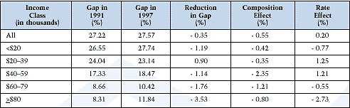 In relative terms, the income gaps narrowed more with each higher income class. For example, the 3.06-percentage-point reduction in the gap for those households with incomes between $40,000 and $59,999 represents a 21-percent reduction in the 1991 gap, whereas the 1.78-percentage-point reduction in the gap for those households with incomes between $60,000 and $79,999 represents a 37-percent reduction. The gap analysis uses the homeownership rate for the highest income households as the standard against which to measure the progress of other groups. This technique implicitly assumes that the highest income households face few, if any, barriers to becoming homeowners, and, therefore, their homeownership rate is the maximum achievable under current conditions and tax laws. One would expect the barriers to be lower as one moves up the income levels; therefore, lower interest rates and improved economic conditions should have the greatest relative impact on higher income households because they face fewer and less severe barriers. The statistics used by HUD to track homeownership on a quarterly and annual basis come from the U.S. Census Bureau and are drawn from the Current Population Survey (CPS). The estimates generated from the CPS include data on minorities and whites, as defined in this article, only from 1994 through 1999. During that period, the difference between the homeownership rate of minorities and whites (the gap) narrowed from 26.8 percentage points in 1994 to 25.5 percentage points in 1999. The AHS presents a different picture for the period 1991 through 1997. In 1991 the gap between minorities and whites as measured by the AHS was 27.22 percentage points. On the basis of demographic trends alone, this gap should have increased by 0.55 percentage points to 27.77 percentage points by 1997. In fact, the actual gap was 27.57 percentage points, 0.35 percentage point more than in 1991 but 0.20 percentage point less than expected based on the changing demographics.5 The first row of table 2 shows how the positive rate effect was insufficient to offset the negative composition effect. Table 2 also shows the interaction between income and race. The homeownership gap between minorities and whites as measured by the AHS increased between 1991 and 1997 for all income classes except for $20,000 to $39,000. In all cases, the composition effect contributed to the widening of the gap. Across the combined income classes, the rate effect helped narrow the gap. The positive rate effect was confined to two income classes, those with incomes between $20,000 and $39,999 and those with incomes between $40,000 and $59,999. It is important to distinguish between the analysis of trends and the analysis of gaps. The previous section showed how the composition effect helped increase the homeownership rate for both minorities and whites. Although the demographic trends helped both groups, they appeared to be more important for whites, accounting for almost half of the increase in the white homeownership rate. This observation is consistent with the results in table 2. When comparing minorities and whites, the demographic trends, as reflected in the composition effect, appear to have caused the gap to widen. Caveats Readers should be aware of three important caveats.
Although the reader should be cautious, given the aforementioned caveats, the AHS does contain a wealth of information that sheds light on what has been happening to homeownership rates. Clearly, both compositional and rate effects have been at work. In general, the rate effects seem to be more important. There has been a strengthening of homeownership rates throughout the population. Both minorities and whites have benefited. The rate effect appears to have been stronger for minorities than for whites, while the composition effect has been stronger for whites than minorities. As measured by the AHS, the gap between minorities and whites has increased but only because the composition effect has outweighed the rate effect. Overall, the rate effect was five times stronger than the composition effect. In addition, substantial progress has been achieved in reducing the income gap, with reductions ranging from 5 percent of the 1991 gap for the lowest income class to 37 percent for the $60,000 to $79,999 class. The impact of the Nation's longest economic expansion is clearly visible in these numbers. Low interest rates and high consumer optimism, based on low inflation and low unemployment, would be reflected in this analysis as rate rather than composition effects.6 The length of the expansion has probably been the most important factor in reducing the income gap. To the extent that lower income households face barriers to homeownership, such as insufficient savings or poor credit ratings, a long recovery allows them to acquire the resources to overcome those barriers.
Because there are approximately 50,000 households in an AHS, sample sizes were small or zero for a number of categories. In these cases, homeownership rates were derived by aggregating adjacent categories.
In this analysis, the term minorities includes all groups except non-Hispanic whites.
Note that the composition effect was substantially smaller for the overall population than for either minorities or whites. An increase in the minority share of the population explains this result.
In relative terms, minorities did show progress. In 1991, the minority homeownership rate was 61.2 percent of the white rate; by 1997, it was 62.0 percent of the white rate—a slight improvement.
Rising income would be incorporated in the composition effects as households shifted from lower income classes to higher income classes.
|
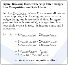 This article uses the AHS to calculate these two effects. First, the AHS sample is desegregated into 1,050 groups defined along five dimensions: age (seven classes), household type (five classes), race (minorities and whites), income (five classes),